---
title: "A Wealth Tax Is a Silent Partner"
description: "The surprising mathematics of proportional wealth taxation — and why your optimal portfolio doesn't change."
author: "Anders G Frøseth"
date: "2026-02-15"
categories: [wealth tax, portfolio theory, asset pricing]
---
## The intuition
Imagine you own a portfolio of stocks, bonds, and other assets. The government introduces a 1% annual wealth tax on the market value of everything you own. Your first instinct might be to restructure your portfolio — perhaps shift toward safer assets, or toward asset classes that are harder to value.
But here's the surprising result: under a cleanly implemented proportional wealth tax, your optimal portfolio doesn't change at all.
## The mathematics
The result depends on three conditions: the tax is levied at a *uniform rate* on *all* assets, assessed at *market value*, in *frictionless markets* (no transaction costs from liquidating to pay the tax). Under these conditions, the tax enters as a single multiplicative factor that scales the entire portfolio identically — which is what drives the neutrality. Relax any one of them and the clean factorisation breaks.
Consider a single-period setting. An investor holds a portfolio with random gross return $R$. Without the wealth tax, terminal wealth is
$$
W_1 = W_0 \cdot R
$$
With a proportional wealth tax at rate $\tau$, the tax is levied on the market value of the portfolio at the end of the period, so terminal wealth after tax becomes
$$
W_1^\tau = W_0 (1 - \tau) \cdot R
$$
The key observation is that $(1 - \tau)$ is a **multiplicative constant** — it scales all outcomes by the same factor. This means:
- **Expected wealth** falls by the factor $(1 - \tau)$
- **Standard deviation of wealth** also falls by exactly $(1 - \tau)$
- The **coefficient of variation** $\sigma / \mu$ is unchanged
- The **Sharpe ratio** of every portfolio is preserved
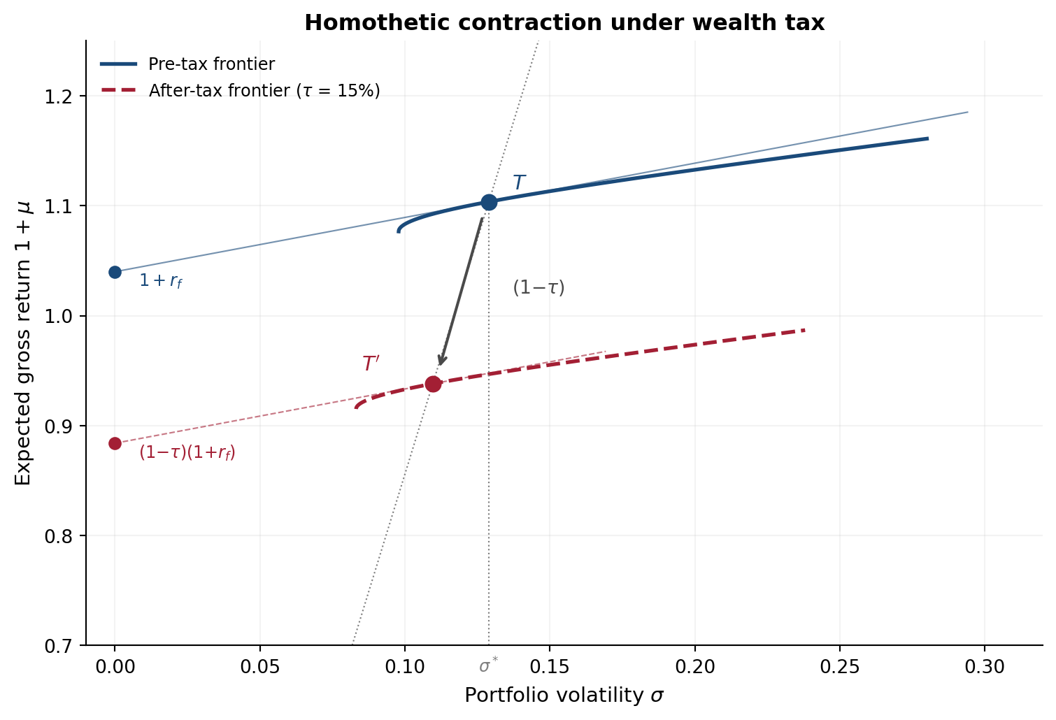
In the mean–standard deviation plane, the wealth tax induces a **homothetic contraction** of the entire opportunity set toward the origin. Every frontier portfolio shrinks proportionally, so the tangency portfolio — the one with the highest Sharpe ratio — remains the same.
## A visual example
Here's what this looks like for a simple two-asset portfolio. We can compute the efficient frontier with and without the tax:
```{python}
#| label: fig-frontier
#| fig-cap: "Homothetic contraction of the efficient frontier under a wealth tax. In the gross-return plane, the tax contracts the entire opportunity set radially toward the origin by the factor $(1-\\tau)$. The tangency portfolio $T$ moves to $T'$ along the ray from the origin — both risk and return shrink proportionally, so the Sharpe ratio is preserved. The tax rate is set to 15% for visual clarity; the geometry is identical at any rate."
#| code-fold: true
import numpy as np
import matplotlib.pyplot as plt

# Parameters
rf = 0.04           # risk-free rate
tau = 0.15          # illustrative tax rate (as in Paper 1, Figure 3)

# Two risky assets
er = np.array([0.07, 0.14])          # expected returns
vol = np.array([0.10, 0.22])         # volatilities
rho = 0.25                            # correlation
cov = np.array([[vol[0]**2, rho*vol[0]*vol[1]],
                [rho*vol[0]*vol[1], vol[1]**2]])

# Efficient frontier (parametric in weight w on asset 1)
w1 = np.linspace(-0.3, 1.2, 500)
port_er = w1 * er[0] + (1 - w1) * er[1]
port_vol = np.sqrt(w1**2*cov[0,0] + (1-w1)**2*cov[1,1]
                    + 2*w1*(1-w1)*cov[0,1])

# Upper branch: keep only the part above the minimum-variance portfolio
min_idx = np.argmin(port_vol)
front_vol = port_vol[:min_idx+1][::-1]     # reverse so sigma increases
front_er  = port_er[:min_idx+1][::-1]

# Tangency portfolio (analytic)
excess = er - rf
cov_inv = np.linalg.inv(cov)
w_tan = cov_inv @ excess
w_tan = w_tan / w_tan.sum()
sigma_tan = np.sqrt(w_tan @ cov @ w_tan)
mu_tan    = w_tan @ er
sharpe    = (mu_tan - rf) / sigma_tan       # slope of the CAL

# After-tax tangency (homothetic contraction)
sigma_tan_tax = (1 - tau) * sigma_tan
mu_tan_tax    = (1 - tau) * (1 + mu_tan)    # gross return

# Plot
fig, ax = plt.subplots(figsize=(8, 5.5))

# Pre-tax frontier (in gross-return space)
ax.plot(front_vol, 1 + front_er, color='#1a4a7a', linewidth=2,
        label='Pre-tax frontier')

# After-tax frontier: homothetic contraction by (1 - tau)
ax.plot((1-tau)*front_vol, (1-tau)*(1+front_er), color='#a31f34',
        linewidth=2, linestyle='--',
        label=f'After-tax frontier ($\\tau$ = {tau:.0%})')

# Capital allocation lines (tangent by construction)
cal_sigma = np.linspace(0, max(front_vol)*1.05, 100)
cal_pretax   = (1 + rf)             + sharpe * cal_sigma
cal_aftertax = (1 - tau) * (1 + rf) + sharpe * cal_sigma

ax.plot(cal_sigma, cal_pretax, color='#1a4a7a', linewidth=0.8, alpha=0.6)
# Trim after-tax CAL near its tangency point
mask_cal = cal_sigma <= sigma_tan_tax + 0.06
ax.plot(cal_sigma[mask_cal], cal_aftertax[mask_cal], color='#a31f34',
        linewidth=0.8, alpha=0.6, linestyle='--')

# Risk-free points
ax.plot(0, 1 + rf, 'o', color='#1a4a7a', markersize=6, zorder=5)
ax.plot(0, (1 - tau) * (1 + rf), 'o', color='#a31f34', markersize=6,
        zorder=5)
ax.text(0.008, 1 + rf, '$1+r_f$', fontsize=9, color='#1a4a7a',
        ha='left', va='top')
ax.text(0.008, (1 - tau) * (1 + rf),
        '$(1{-}\\tau)(1{+}r_f)$', fontsize=9,
        color='#a31f34', ha='left', va='top')

# Tangency points
ax.plot(sigma_tan, 1 + mu_tan, 'o', color='#1a4a7a', markersize=8,
        zorder=5)
ax.plot(sigma_tan_tax, mu_tan_tax, 'o', color='#a31f34', markersize=8,
        zorder=5)
ax.text(sigma_tan + 0.008, 1 + mu_tan + 0.012, '$T$', fontsize=11,
        color='#1a4a7a', fontweight='bold')
ax.text(sigma_tan_tax - 0.018, mu_tan_tax + 0.012, "$T'$", fontsize=11,
        color='#a31f34', fontweight='bold', ha='right')

# Dotted ray from origin through tangency points
ray_end_sigma = sigma_tan * 1.15
ray_end_mu    = ((1 + mu_tan) / sigma_tan) * ray_end_sigma
ax.plot([0, ray_end_sigma], [0, ray_end_mu], ':', color='gray',
        linewidth=0.8)

# Arrow showing radial contraction
ax.annotate('', xy=(sigma_tan_tax + 0.002, mu_tan_tax + 0.012),
            xytext=(sigma_tan - 0.002, 1 + mu_tan - 0.012),
            arrowprops=dict(arrowstyle='->', color='#4a4a4a', lw=1.5))
ax.text(sigma_tan + 0.008, (1 + mu_tan + mu_tan_tax) / 2,
        '$(1{-}\\tau)$', fontsize=10, color='#4a4a4a')

# Dotted vertical at sigma*
ax.plot([sigma_tan, sigma_tan], [0.7, 1 + mu_tan], ':', color='gray',
        linewidth=0.8)
ax.text(sigma_tan, 0.69, '$\\sigma^*$', fontsize=9, color='gray',
        ha='center', va='top')

ax.set_xlabel('Portfolio volatility $\\sigma$', fontsize=11)
ax.set_ylabel('Expected gross return $1 + \\mu$', fontsize=11)
ax.set_title('Homothetic contraction under wealth tax',
             fontsize=12, fontweight='bold')
ax.legend(fontsize=9, frameon=False, loc='upper left')
ax.set_xlim(-0.01, 0.32)
ax.set_ylim(0.7, 1.25)
ax.spines['top'].set_visible(False)
ax.spines['right'].set_visible(False)
ax.grid(True, alpha=0.15)

plt.tight_layout()
plt.show()
```
The tangency portfolio weight $w^*$ is identical in both cases — the tax doesn't change which portfolio is optimal. It only changes how much wealth you end up with.
## The silent partner analogy
The wealth tax is mathematically equivalent to the government becoming a **silent partner** in your portfolio. Each year, the state claims a $\tau$ fraction of your holdings — as if it owns $\tau$ percent of every share you hold. Your return per share is unaffected; you simply hold fewer shares after the tax.
This is the core insight of the [neutrality framework](/research/wealth-tax/index.qmd).
## When does this break down?
In practice, wealth taxes are never this clean. The [seven channels of distortion](/research/wealth-tax/index.qmd#channels) identified in the framework show exactly how and why real wealth taxes depart from neutrality — from non-uniform assessment fractions to the amplification effects of inelastic markets.
The neutrality result is not an argument for or against wealth taxes. It is a **benchmark** — a precisely defined starting point from which to measure the actual distortions introduced by any specific implementation.